- Myung, I. J., Pitt, M. A. & Kim, W. (2003). Model Evaluation, Testing, and Selection. In: K. Lamberts and R. Goldstone (Eds.), Handbook of Cognition. London: Sage.
- Morgan textbook:
Chapter 1, especially (or even exclusively) Examples 1.1 and 1.3.
- Busemeyer, J. (in preparation). Working manuscript for textbook on model fitting and comparison. Chapters 1 and 2.
- Navarro, D. J. & Myung, I. J. (2003). Model Evaluation and Selection. Manuscript for encyclopedia article.
- Zucchini, W. (2000). An Introduction to Model Selection. Journal of Mathematical Psychology, 44, 41-61.
No classes Monday Jan. 19: MLK Jr. Day.
- Myung, I. J. (2003). Tutorial on maximal likelihood estimation. Journal of Mathematical Psychology, 47, 90-100.
|
|
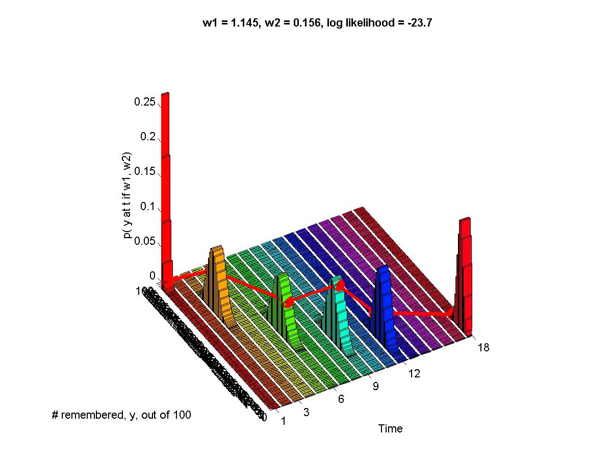
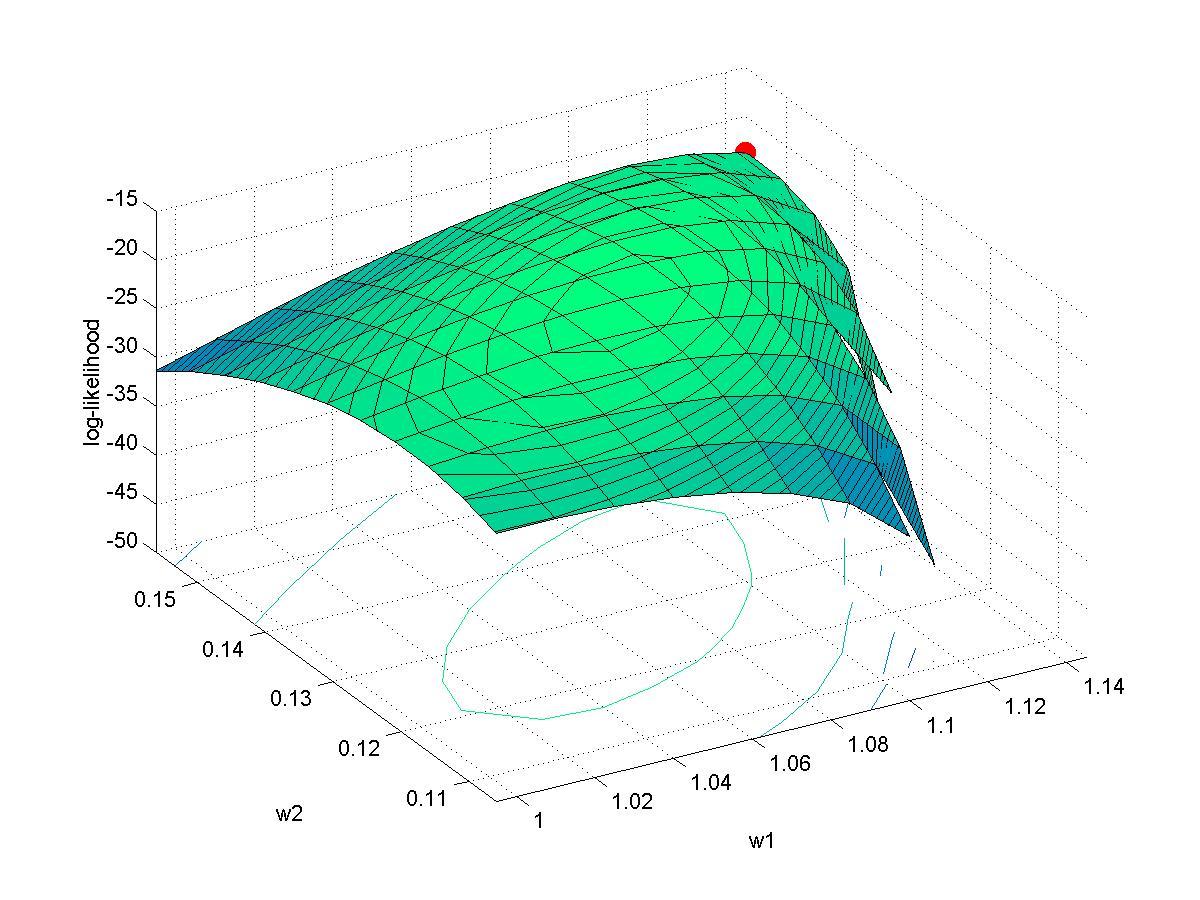
| Left panel shows a predicted sampling distribution from the memory retention model p(t) = w1 exp( -w2 t ), with n=100 at each retention time. An actual sample's data rides (in red dots connected by red lines) atop the predicted sampling distribution. The right panel shows the log-likelihood of the data for different parameter values. Matlab programs and figures by Prof. Kruschke. | |
- Busemeyer, J. (in preparation). Working manuscript for textbook on model fitting and comparison. Chapter 3.
|
|
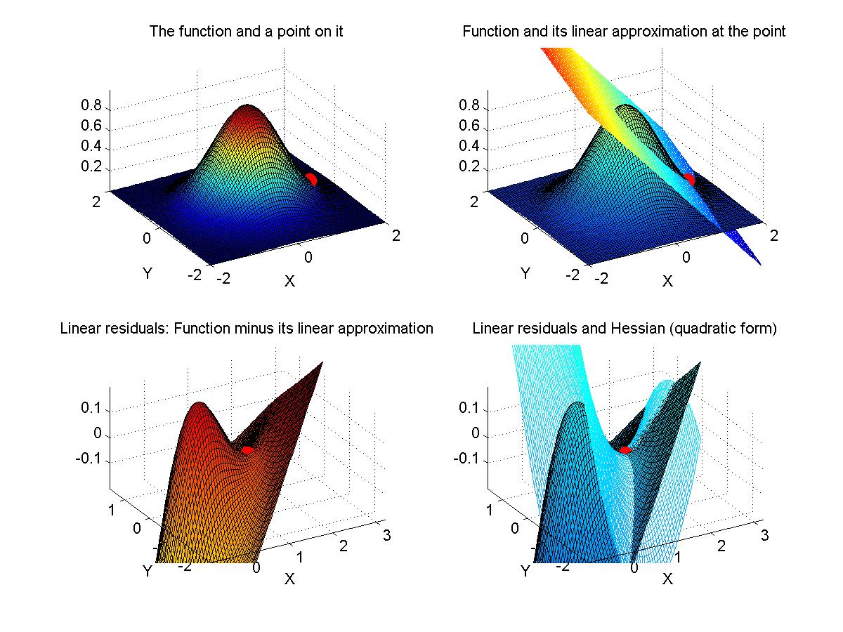
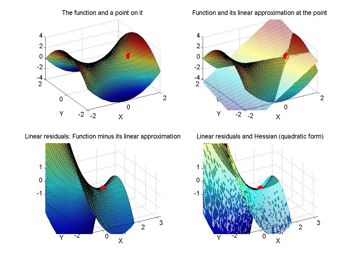
| Each figure above (click to enlarge) shows a function R2 -> R with the linear approximation at a point and the Hessian approximation to the residuals. The left figure shows a Gaussian function and the right figure shows a quadratic. Notice in the right figure that the Hessian matches the linear residuals, to within limits of numerical approximation. The Matlab program that generated these graphs was written by Prof. Kruschke. | |
- Morgan textbook:
Chapter 2; specifically section 2.2, regarding an example of an analytical solution to a maximal likelihood estimation problem.
Chapter 3: Function optimization methods.
If time, we'll go back to Myung (2003) and look at his Matlab programs for maximal likelihood estimation. - Assignment: The goal of this assignment is for you to learn about the linear and Hessian approximations to a likelihood function. A secondary goal is for you to limber up your Matlab fingers. The assignment is for you to compose Matlab programs that can make graphs like those shown above. That is, for a given function of two variables, plot the function, its linear approximation at a point, its residuals, and the Hessian approximation to the residuals at that point. Due Monday February 9.
- Busemeyer, J. (in preparation). Working manuscript for textbook on model fitting and comparison. Chapter 3.
|
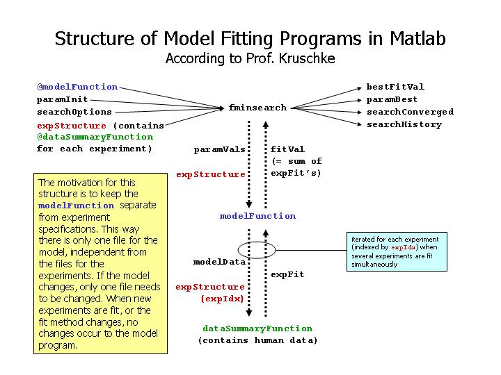
| Structure of model fitting programs in Matlab, as advised by Prof. Kruschke. |
- Morgan textbook Chapter 3: Understanding the Newton-Raphson method and Hessian matrices. Example of likelihood optimization in Matlab for Fig. 3.4.
- Myung (2003): Example of MLE fit to memory retention data, and Matlab code.
- Busemeyer, J. (in preparation). Working manuscript for textbook on model fitting and comparison. Chapter 3 and its Appendix.
- Assignment: The goal of this assignment is for you to
get experience with model fitting in Matlab.
The file BusemeyerRetentionModelData.txt, posted in Oncourse, contains simulated data for a retention experiment like that described by Busemeyer in his Chapter 3. The file contains one row per trial, with each row specifying the Subject number, Duration (in seconds), the Trial number (for that duration for that subject), and the Recall success (1 for successful recall, 0 for failure to recall). As you can see by examining the file, there are 10 subjects, 5 different durations, and 50 trials per duration.
Your job is to fit the retention model (Equation 4, Page 9, Chapter 3 of Busemeyer's draft textbook) to each individual subject's data (i.e, using different parameter values for each subject), and to fit the model simultaneously to all the subjects (i.e., using a single set of parameter values to best fit all the data simultaneously).
Use maximal likelihood as your measure of fit. That is, minimize the negative log-likelihood.
Structure your files the way Prof. Kruschke recommends (see diagram above), putting the model in a file separate from the file that specifies the experiment design and data and fit function. An example of this sort of structure was described in class on Monday Feb. 9 and can be found in Oncourse under the "In Touch" tab, "Group Spaces" link "Matlab Programs", then in the folder "ForMyung2003". The model is specified in the file "ExpMemModel.m" and the experiment and data etc. are specified in the file "Murdock61_ExpMemModel.m". The log-likelihood computation also calls the function specified in "choose.m".
Due Monday Feb. 16, by class time.
|
|
|
|
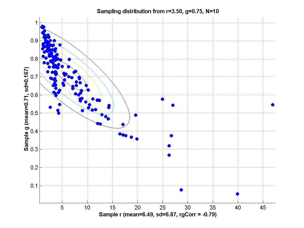
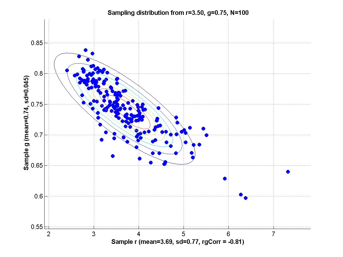
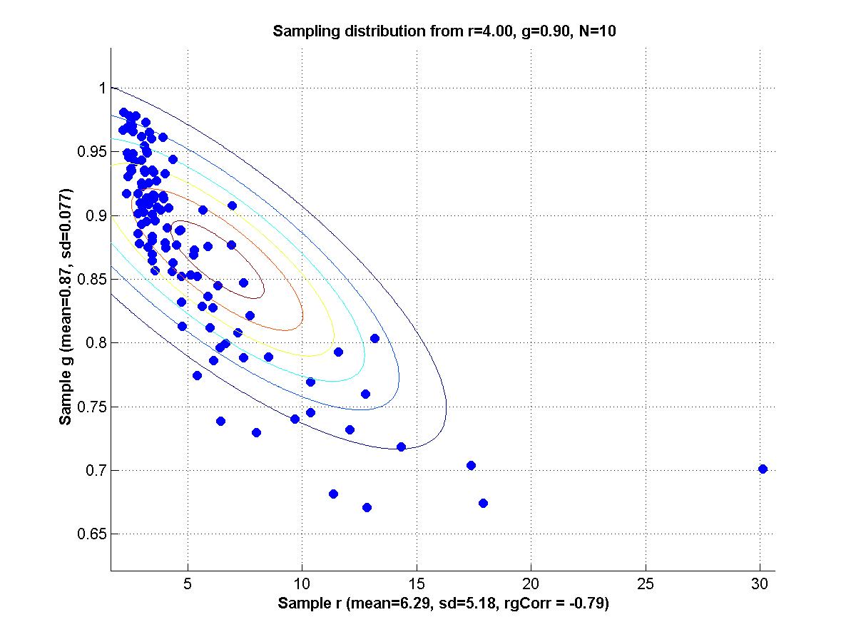
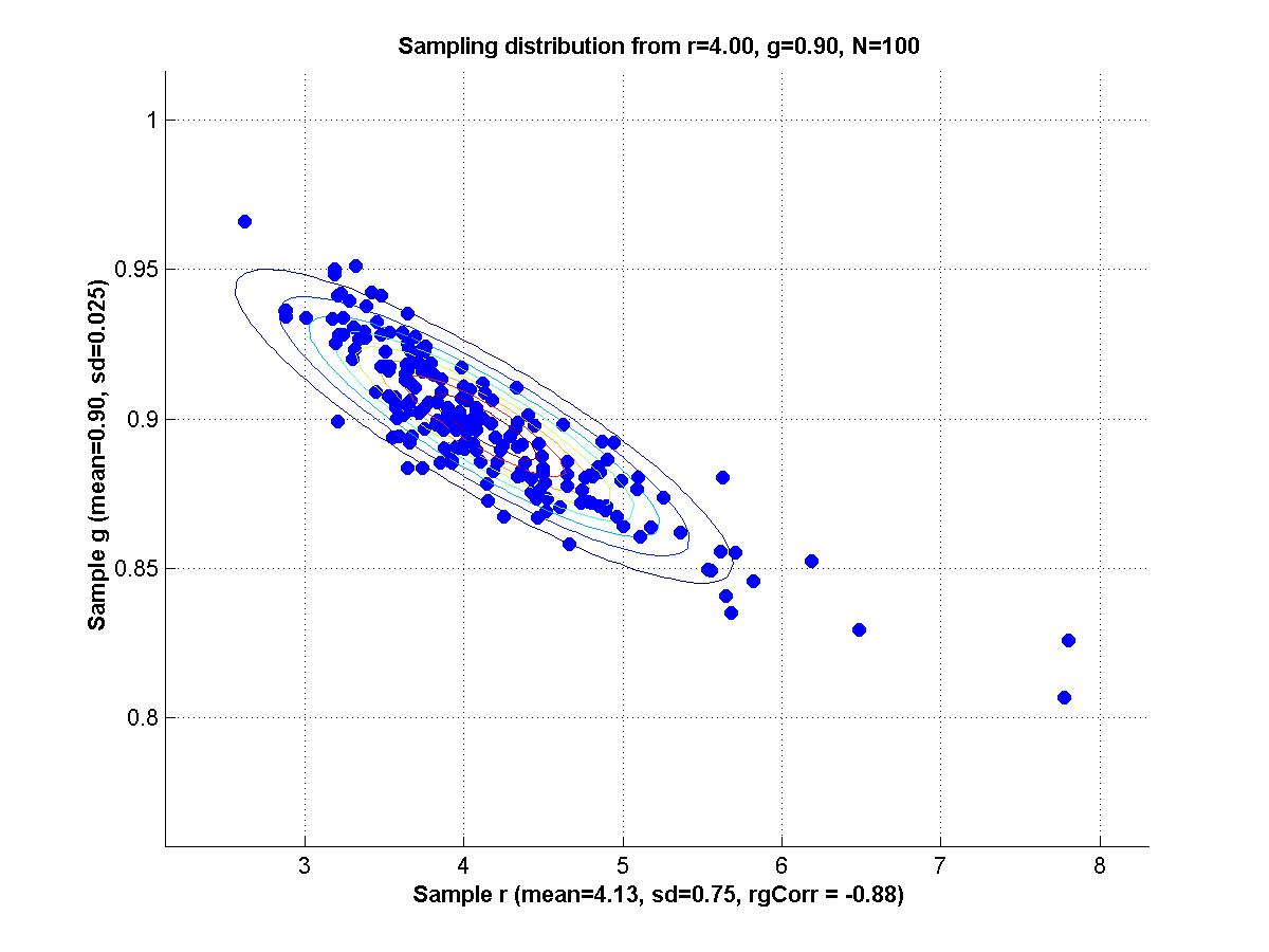
| Sampling distributions of maximal likelihood estimates of parameters for the "toy" memory retention model p(t) = 1/(1+exp(-r gt)). Level contours show bivariate normal with same means and covariance as the sampling distribution. Rows are for different populations sampled from. Columns are for different sample sizes. Click on any panel to enlarge. Matlab programs and graphs by Prof. Kruschke. | |
Readings:
- Ch. 4 of Morgan textbook. (Unfortunately I'm discovering that the Morgan textbook is unsuitable as an initial tutorial on these topics; it might be better as a reminder or review for people already familiar with the details. Nevertheless, give it a go and I'll do a lot of derivations in class.)
|
|
|
|
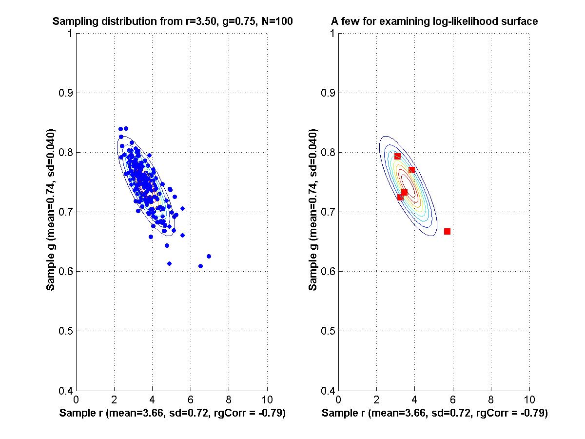
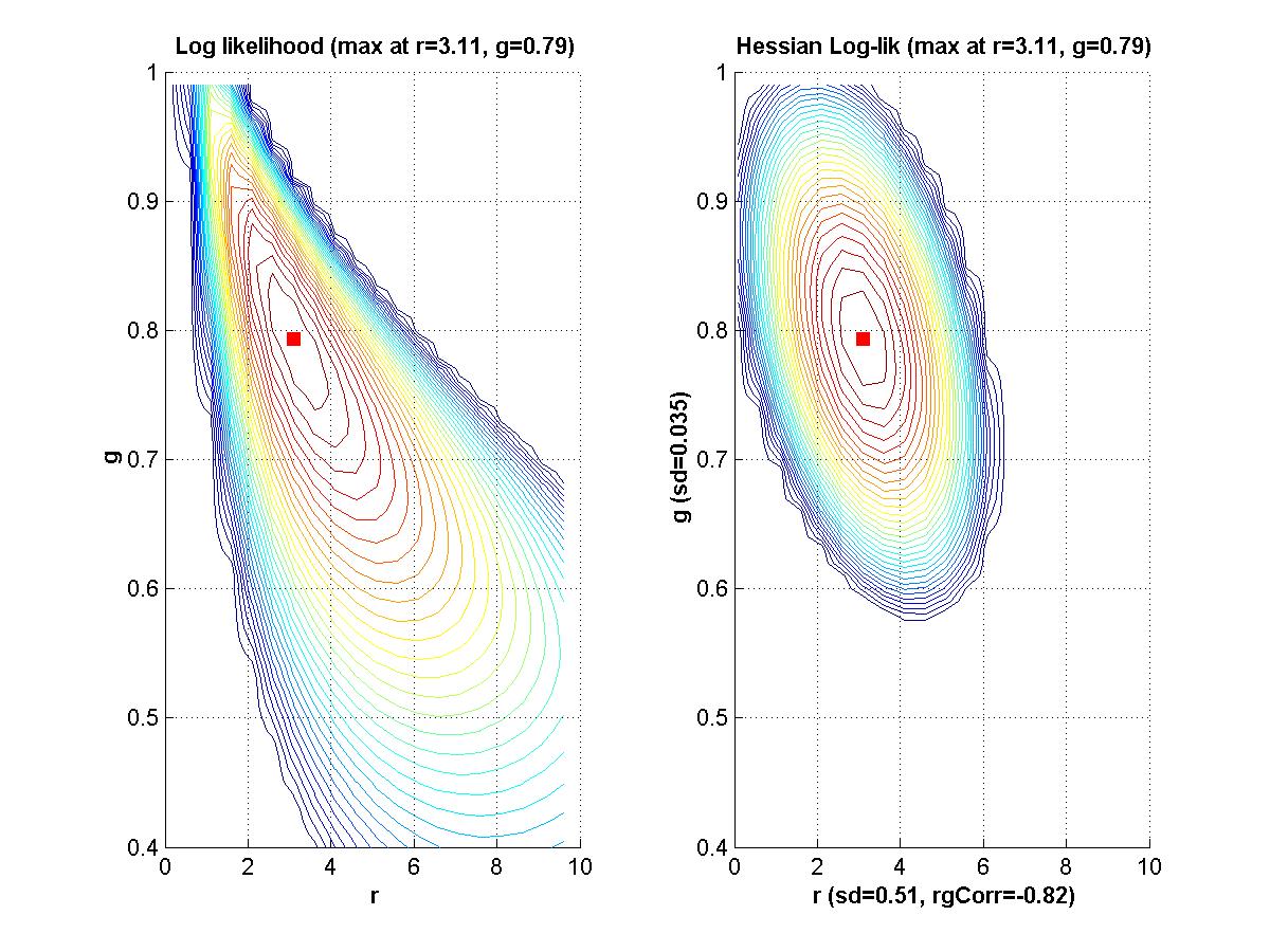
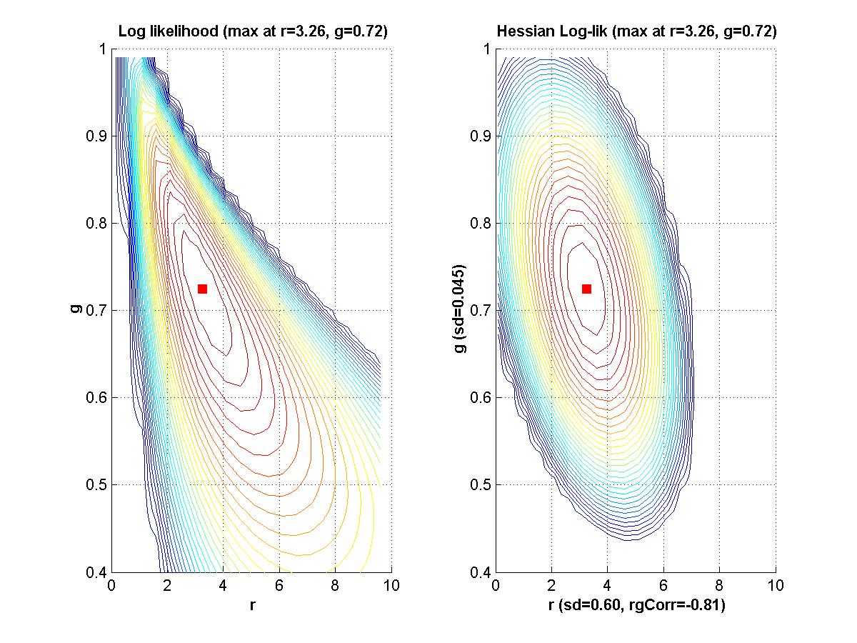
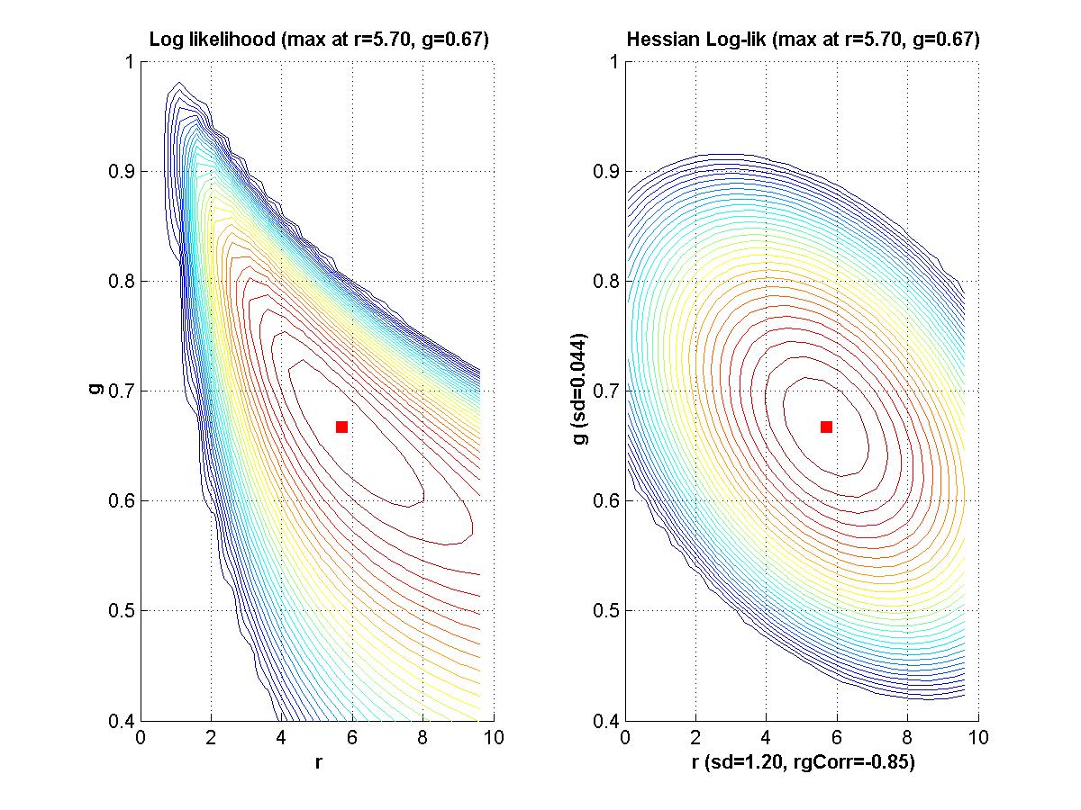
| Top left: Sampling distribution of maximal likelihood estimates for large N (this is same as the top right graph in last week's figure, rescaled). The other three panels show three specific samples' actual likelihood surfaces and Hessian approximations. Confidence regions can be constructed from the likelihood contours; approximate confidence regions can be constructed from the Hessian approximations. Matlab programs and graphs by Prof. Kruschke. | |
- Verguts, T. and Storms, G. (2003?). Assessing the informational value of parameter estimates in cognitive models. Unpublished manuscript.
- Busemeyer, draft textbook, Chapter 4 and Appendix.
- Ratcliff, R. and Tuerlinckx, F. (2002). Estimating parameters of the diffusion model: Approaches to dealing with contaminant reaction times and parameter variability. Psychonomic Bulletin and Review, 9(3), 438-481.
- Huber, D. E. (2003?). Computer simulations of the ROUSE model: An analytic method and a generally applicable technique for producing parameter confidence intervals. Unpublished manuscript.
- Wichmann, F. A. and Hill, N. J. (2001). The psychometric function: II. Bootstrap-based confidence intervals and sampling. Perception and Psychophysics, 63(8), 1314-1329.
- This assignment follows from the Verguts and Storms
manuscript. The purpose is to explore whether the parameter redundancy
(or lack of redundancy) discovered by parameter fitting can be derived
algebraically.
Show algebraically that, in ALCOVE, the specificity parameter ("c") and the attention learning rate parameter ("lambda_alpha") exactly trade off. That is, show that when one parameter is "twiddled" a small amount, an exactly compensating twiddle can be made in the other parameter. The relevant equations for the ALCOVE model can be found in the file Kruschke1992.pdf in the Readings Group Space, especially Eqn. 6, p. 24.
Next, show that, in RASHNL, the specificity parameter and the gain shift rate parameter do not trade off. See the file KruschkeJ1999.pdf in the Readings; especially Eqn. 7 on p. 1097.
This is due in class Monday March 22. -
This assignment follows-up on the linear regression example in
Ratcliff and Tuerlinckx. Consider the model
y = m * x + b + N(0,1) where m and b are parameters and N(0,1) is a normal distribution with mean zero and standard deviation 1. For all the scenarios below, a sample is generated by 20 cases for each of x = {1,3,5,7,9}; i.e., 100 data points total in a sample.
1. Set m = 1 and b = 1 as true population parameters. Generate 200 random samples from this population, and for each sample use maximal likelihood estimation to determine mest and best. Make a scatter plot of the sampling distribution of mest and best. Compute the mean of mest and best, and compare with the true values. Compute the SD of mest and best, and the correlation of mest with best.
2. Repeat part 1 but with contaminated samples, as follows. Generate a sample as before, but then for each individual data point retain it, as is, with 92% probability, but replace it, with 8% probability, with a value randomly sampled from a uniform distribution over the interval [0,20]. Compare the new mean mest and mean best with both the true values and the means obtained from uncontaminated samples. Comment also on the SDs and correlation, compared with uncontaminated samples.
3. Reparameterize the model as follows:
y = (m+b) * x + (b-m) + N(0,1) Repeat part 1; i.e., with uncontaminated samples. Now the generating model again has the slope and intercept equal to 1; that is, (m+b)=1 and (b-m)=1, which implies that m=0 and b=1. Comment on the correlation of mest and best for the reparameterized model, compared with the original model.
Due Monday March 29 in class.
Readings regarding the generalized likelihood ratio test (G2) for nested models:
- Busemeyer Ch. 3, pp. 39-41.
- Busemeyer Ch. 4, pp. 22-26.
- Busemeyer Ch. 5, pp. 25-29.
|
|
|
|
|
|
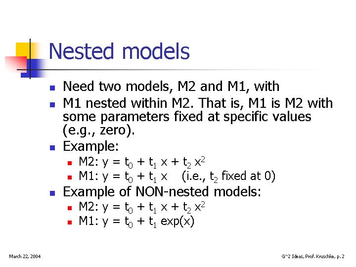
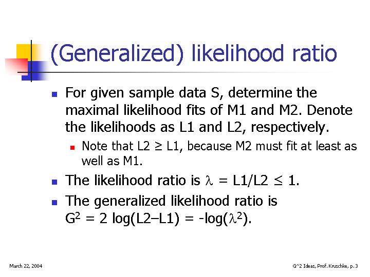
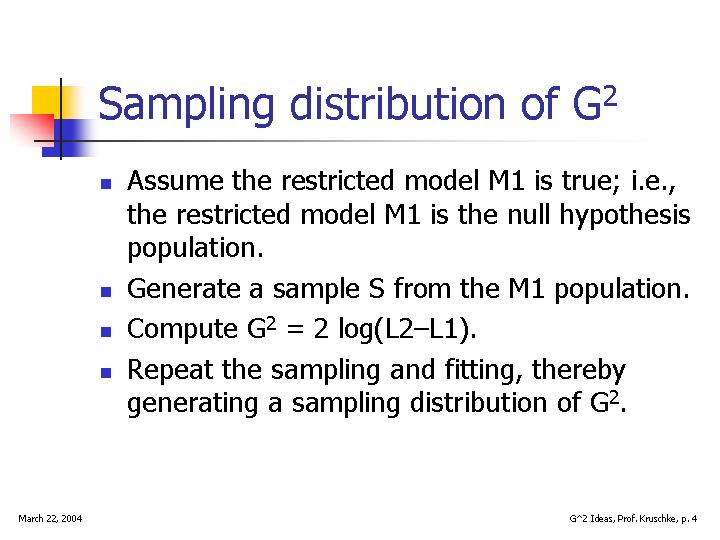
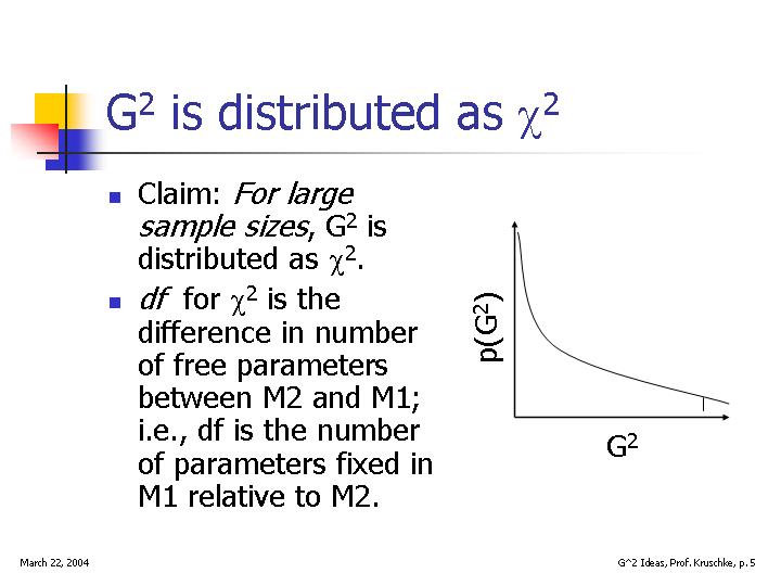
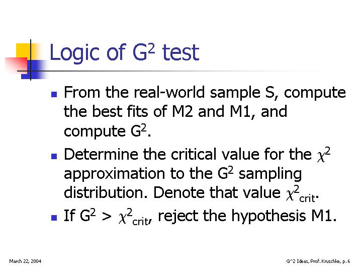
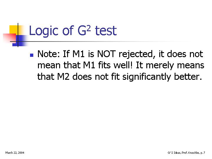
| Selected lecture overheads regarding G2. I hope the information here is approximately correct; treat it as a noisy sample. | |
|
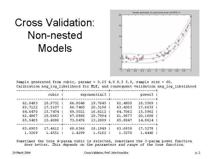
|
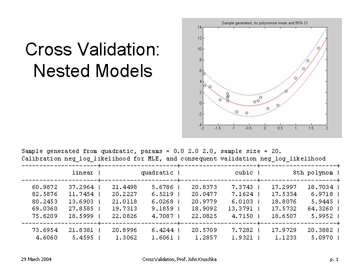
| Selected lecture overheads regarding cross validation. | |
Reading: Busemeyer and Wang (2000). Model comparisons and model selections based on generalization criterion methodology. Journal of Mathematical Psychology, 41, 171-289.
Readings:
- Myung and Pitt (1997).
- David J. C. MacKay (1991 NIPS).
- David J. C. MacKay (199X Network article).
Readings: Continuation from last week.
- Myung and Pitt (1997).
- David J. C. MacKay (1991 NIPS).
- David J. C. MacKay (199X Network article).
|
|
|
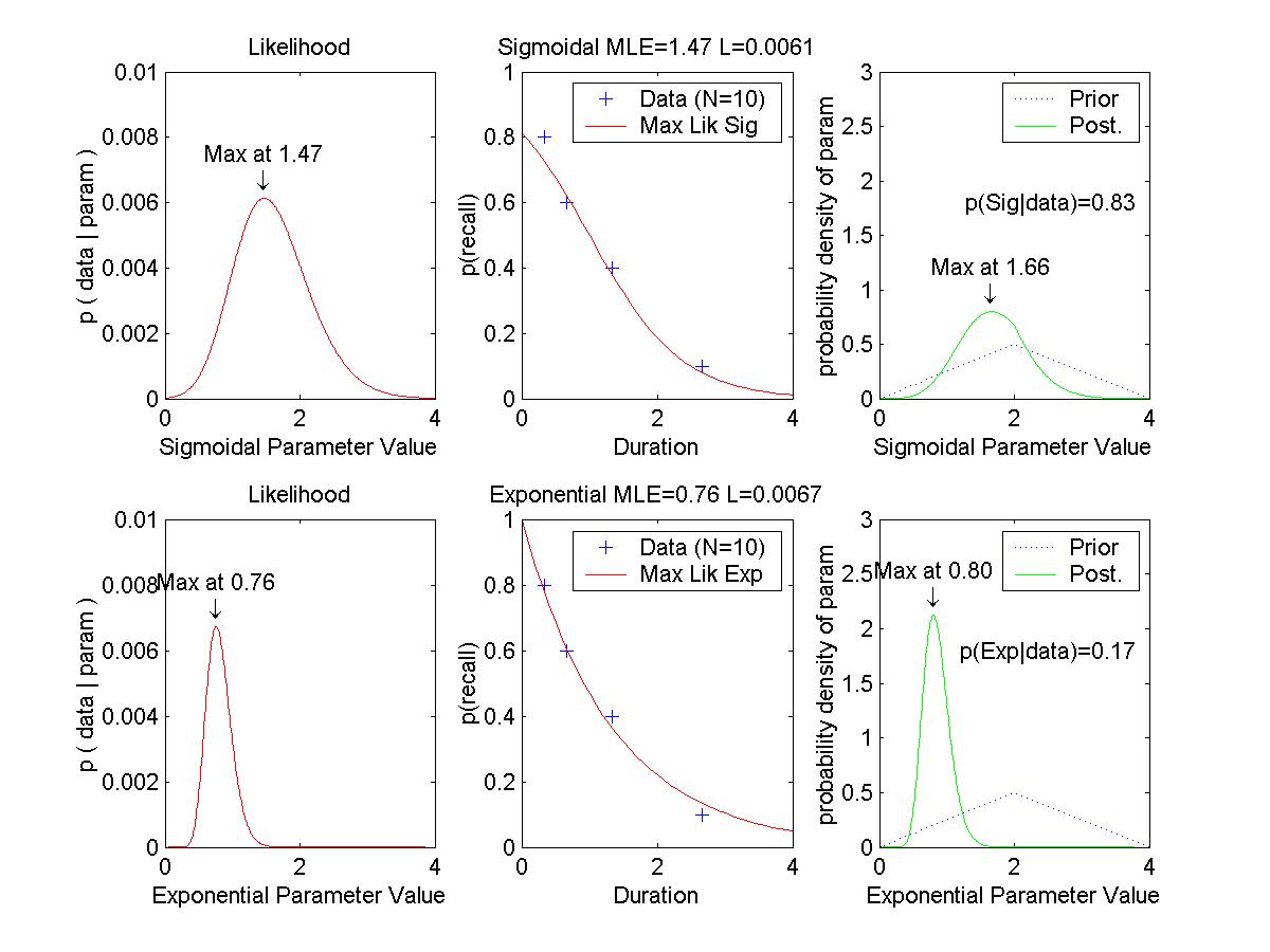
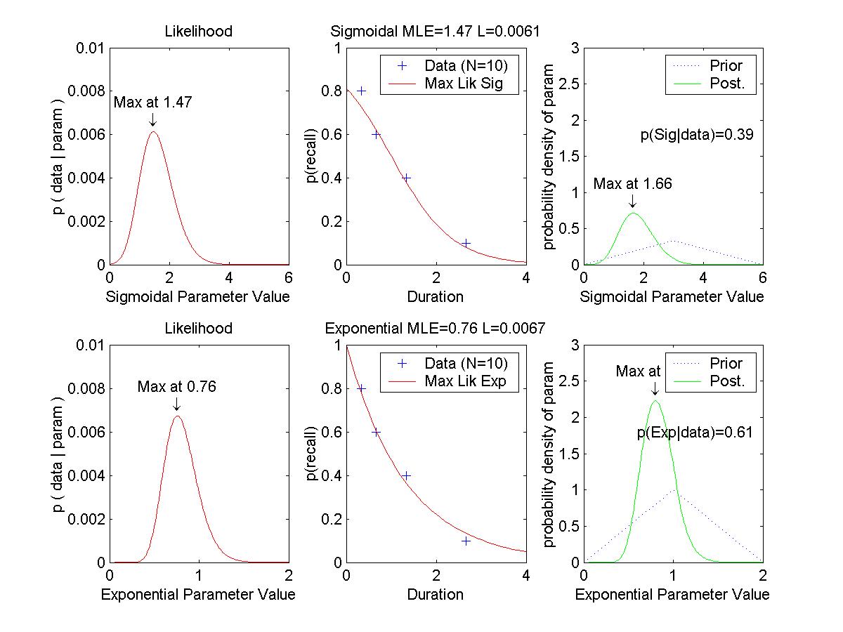
Bayesian parameter estimation and model comparison for two "toy"
retention models: Exponential: p(x) = exp( -a * x ), and Sigmoidal: p(x) = 1 ./ ( 1 + exp( b * ( x - 1 ))). The left panel above shows a case of "equal" prior distributions across the two parameters, with the result being a higher posterior probability for the Sigmoidal model. The right panel shows a case of different ranges for the priors of the two parameters, with the result being a higher posterior probability for the Exponential model. These graphs are generated by evaluating the model at many finely-spaced increments of the parameter. For multi-parameter models that are also time-consuming to evaluate even once, generating analogous graphs or computations could be impossible in practice. Matlab program and graphs by Prof. Kruschke. |
|
Optional Assignment: (Essentially, make the graphs shown above.) Consider two "toy" memory retention models, which predict the probability (p) of recall as a function of duration (x, in some unspecified time scale):
H1, exponential: p(x) = exp( -a * x )Each model has a single parameter, a and b respectively. We assume that for any given duration x, when a subject tries to recall an item, the probability of success is p(x) and is independent of other trials; i.e., the sampling distribution of successful recall is distributed as a binomial distribution with probability p(x).
H2, sigmoidal: p(x) = 1 ./ ( 1 + exp( b * ( x - 1 )))
| Duration | 0.33 | 0.67 | 1.33 | 2.67 |
|---|---|---|---|---|
| Proportion recall |
0.8 | 0.6 | 0.4 | 0.1 |
(A) Determine the maximal likelihood estimates of a and b for the two models. This is merely the sort of thing we did in previous weeks; we are maximizing p(data|a,hyp_a) and p(data|b,hyp_b). Graph the likelihood functions. Graph the data points superimposed with the curves of p(x) for these "best fitting" models.
(B) Suppose that we have identical "triangular" prior probability distributions over the two parameters, such that
p(a|hyp_a) = (1/2) - abs( (1/4) * ( a - 2.0 ) ), 0 <= a <= 4.0.Determine the posterior probability distributions over the two parameters, given the data above. Use Eqn's 3 and 6 of MacKay's chapter:
p(b|hyp_b) = (1/2) - abs( (1/4) * ( b - 2.0 ) ), 0 <= b <= 4.0.
p(a|data,hyp_a) = p(data|a,hyp_a) p(a|hyp_a) / p(data|hyp_a) [Eqn. 3]When integrating for Eqn. 6, use numerical approximation. That is, finely divide the range of a into delta_a's, compute p(data|a) and p(a) at each point, and sum (integrate) them up across points. Don't forget to include delta_a in the product you are summing. Graph the prior and posterior distributions (superimposed). Is the maximum of each posterior close to the maximal likelihood estimate of the corresponding parameter?
p(data|hyp_a) = Integral_a p(data|a,hyp_a) p(a|hyp_a) delta_a [Eqn. 6]
(C) Suppose that the prior probabilities of the models are equal; i.e., p(hyp_a) = p(hyp_b) = 0.5. Determine the posterior probabilities of the models, given the data. Use the equations
p(hyp_a|data) = p(data|hyp_a) p(hyp_a) / p(data)and Eqn. 6, above.
p(data) = p(data|hyp_a) p(hyp_a) + p(data|hyp_b) p(hyp_b)
Pitt, Myung and Zhang (2002). Toward a method of selecting among computational models of cognition. Psychological Review, 109, 472-491.